Profile Resampling (‘microslicing’)#
The Nevot-Croce roughness approximation only strictly holds for cases where the interface roughness is much less than the layer thickness. The usual way of handling cases where this approximation does not hold is to split the interfaces into a large number of layers of zero roughness, so that the roughness problem is circumvented:
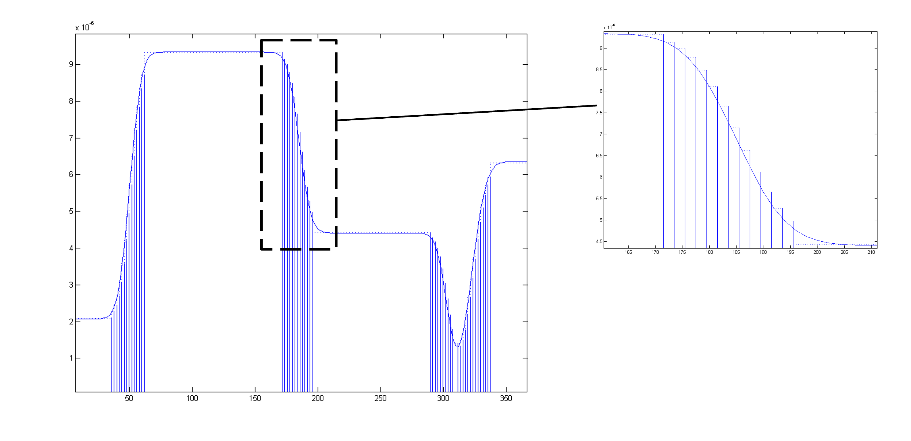
However, this kind of “dumb microslicing” causes the creation of a large number of layers, which may not all be necessary and will significantly slow down the calculation.
This problem of finding the lowest number of individual points that will completely describe a waveform is a common problem in signal processing. RAT uses a technique borrowed from signal processing called Adaptive Resampling (AR).
AR is an interactive process which aims to find the lowest number of points that will best describe a curve. It does this by adding points where the angle between neighbouring points becomes smaller than a threshold value. So, it adds more points where the signal is changing most strongly (in order to capture all details of the curvature). So, for a cosine wave, the resampled points cluster at the regions of the largest curvature:
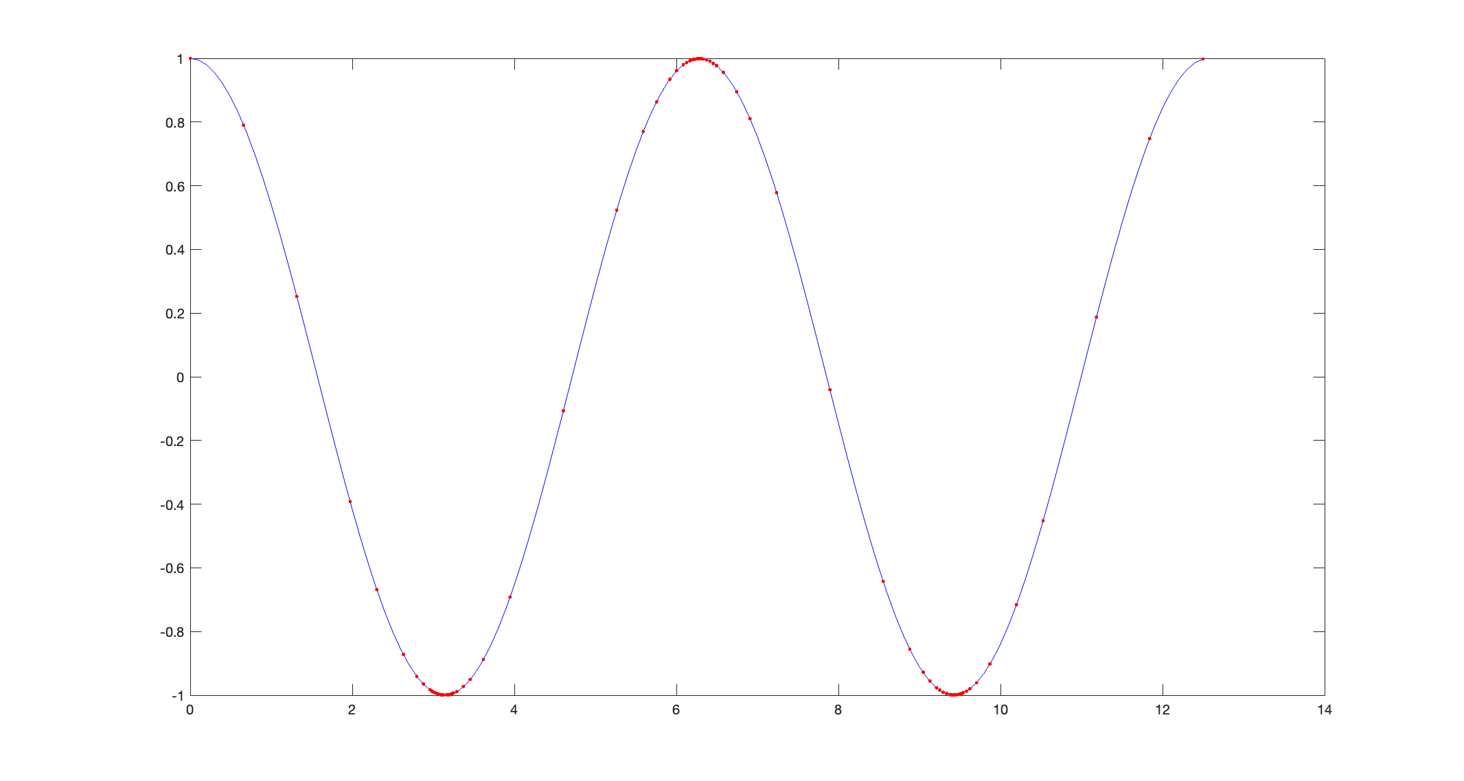
For the continuous cosine curve shown in blue, the AR algorithm has chosen the red points as being most representative. In other words, if the red points were joined with straight lines, the resulting curve would be very similar to the original signal. The salient point is that more points are required where the gradient of the signal is changing quickly, and those where the gradient is constant can be represented by fewer points.
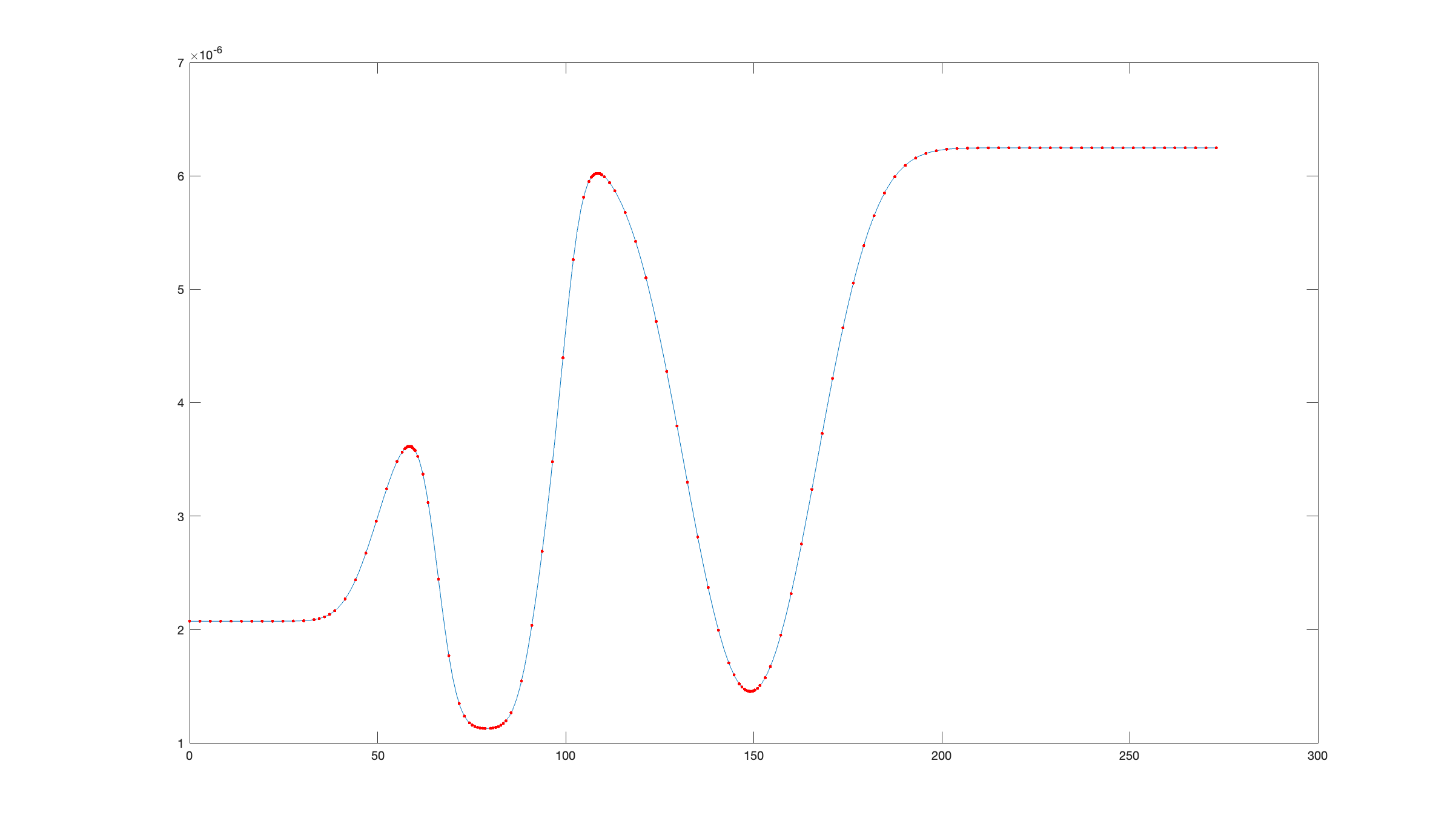
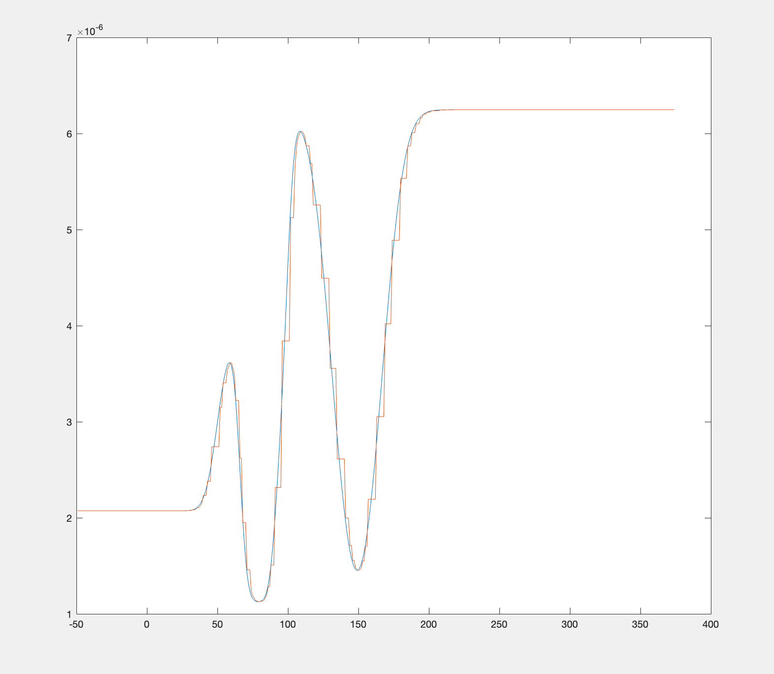
RAT borrows the AR trick from the signal processors, and uses this method to resample the SLD profiles. The AR algorithm is used to find the best series of points that will represent the profile most accurately, and then each of these points is taken as the centre of the layer (of zero roughness). The thickness of each layer is half the distance between neighbouring points. So, for an SLD profile of a floating bilayer (blue line), AR selects the red points:
which are then converted into a set of zero roughness layers:
Using Resampling in RAT#
Using resampling on a contrast in RAT is very simple. For any contrast that you want to resample, simply set the resample flag for that contrast as shown below:
problem.setContrast(1, 'resample', true);
problem.contrasts.set_fields(0, resample=True)
             p                        1                          2
    ___________________    _______________________    ________________________

    "Name"                 "D-tail/H-Head/D2O"        "H-tail/D-Head/ACMW"
    "Data"                 "D-tail / H-head / D2O"    "H-tail / D-head / ACMW"
    "Background"           "Background D2O"           "Background ACMW"
    "Background Action"    "add"                      "add"
    "Bulk in"              "SLD Air"                  "SLD Air"
    "Bulk out"             "SLD D2O"                  "SLD ACMW"
    "Scalefactor"          "Scalefactor 1"            "Scalefactor 1"
    "Resolution"           "Resolution 1"             "Resolution 1"
    "Resample"             "true"                     "false"
    "Repeat Layers"        "1"                        "1"
    "Model"                "Deuterated Tails"         "Hydrogenated Tails"
    ""                     "Hydrogenated Heads"       "Deuterated Heads"
+-------+--------------------+-----------------------+-----------------+-------------------+---------+----------+---------------+--------------+----------+---------------+--------------------+
| index |        name        |          data         |    background   | background action | bulk in | bulk out |  scalefactor  |  resolution  | resample | repeat layers |       model        |
+-------+--------------------+-----------------------+-----------------+-------------------+---------+----------+---------------+--------------+----------+---------------+--------------------+
|   0   | D-tail/H-Head/D2O  | D-tail / H-head / D2O |  Background D2O |        add        | SLD Air | SLD D2O  | Scalefactor 1 | Resolution 1 |   True   |       1       |  Deuterated Tails  |
|       |                    |                       |                 |                   |         |          |               |              |          |               | Hydrogenated Heads |
|   1   | H-tail/D-Head/ACMW | D-tail / H-head / D2O | Background ACMW |        add        | SLD Air | SLD ACMW | Scalefactor 1 | Resolution 1 |  False   |       1       | Hydrogenated Tails |
|       |                    |                       |                 |                   |         |          |               |              |          |               |  Deuterated Heads  |
+-------+--------------------+-----------------------+-----------------+-------------------+---------+----------+---------------+--------------+----------+---------------+--------------------+
The resampling operation is controlled by the parameters resampleMinAngle and resampleNPoints in the controls object:
  controlsClass with properties:

               parallel: 'single'
              procedure: 'calculate'
                display: 'iter'
    numSimulationPoints: 500
       resampleMinAngle: 0.9000
        resampleNPoints: 50
+---------------------+-----------+
|       Property      |   Value   |
+---------------------+-----------+
|      procedure      | calculate |
|       parallel      |   single  |
| numSimulationPoints |    500    |
|   resampleMinAngle  |    0.9    |
|   resampleNPoints   |     50    |
|       display       |    iter   |
+---------------------+-----------+
resampleMinAngle: For each data point, the algorithm draws two lines from that data point to its neighbouring points on either side. If the angle between those lines is smaller thanresampleMinAngle, then the algorithm will refine over that point.In practice, this means that resampling happens for points which are significantly higher or lower than their neighbours (i.e. the gradient of the function has changed rapidly) and
resampleMinAnglecontrols the sensitivity of this.resampleMinAngleis defined in the units of ‘radians divided by pi’, i.e.resampleMinAngle = 0.9refines where the adjacent points form an angle smaller than \(0.9 \pi\) radians.resampleNPoints: The initial number of domain points (layers) sampled by the algorithm at the start.
Note
Generally, resampleMinAngle has a larger effect on the eventual resampling than resampleNPoints.
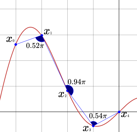
Fig. 2 A simple example of how resampling calculates angles, with resampleNPoints = 5.
If resampleMinAngle were set to its default value of 0.9,
then resampling would occur around \(x_1\) and \(x_3\), but not \(x_2\).#