DSPC Custom XY

This shows an example of using a custom XY model to analyse reflectivity from a supported bilayer of DSPC.

Similar to DSPC Custom Layers, we can make use of the fact that the volumes, and of course the atomistic composition are known. So, for lipid tails for example, then we can take a literature value for the tails volume, have a fittable parameter for the lipid area per molecule, and then the tail thickness will simply be

\[\text{Tail Thick} = \frac{\text{Tail Volume}}{\text{Lipid APM}}.\]

Since the volume is known, then the SLD of the tails is also obviously easily calculable.

In this model, we make distributions to represent the volume fractions of each of the components in the sample, the convert these to SLDs, as described in [1].

We also make our volume fractions as optional outputted parameters from our file. The optional nature of this output means we can suppress it to run the model, then activate it to make final output plots of our analysis.

This example can be run as a script or interactively using the instructions below.

Note

The custom model used is a MATLAB model - examples/normalReflectivity/customXY/customXYDSPC.m.

Run Script:

root = getappdata(0, 'root');
cd(fullfile(root, 'examples', 'normalReflectivity', 'customXY'));
customXYDSPCScript

Run Interactively:

root = getappdata(0, 'root');
cd(fullfile(root, 'examples', 'normalReflectivity', 'customXY'));
edit customXYDSPCSheet.mlx

[1] Shekhar et al, J. Appl. Phys, 100, 102216 (2011) [DOI 10.1063/1.3661986]

Custom XY Example for Supported DSPC layer.

In this example, we model the same data (DSPC supported bilayer) as the Custom Layers example, but this time we will use continuous distributions of the volume fractions of each component to build up the SLD profiles (as described in Shekhar et al, J. Appl. Phys., 110, 102216 (2011). )

In this type of model, each 'layer' in the sample is described by a roughened Heaviside step function (really, just two error functions back to back). So, in our case, we will need an oxide, a (possible) intervening water layer, and then the bilayer itself.

We can define our lipid in terms of an Area per Molecule, almost in it's entirety, if we recognise that where the volume is known, the thickness of the layer is simply given by the layer volume / APM

.

We can then define the Volume Fraction of this layer with a roughened Heaviside of length dlayer and a height of 1. Then, the total volume occupied will be given by the sum of the volume fractions across the interface. Of course, this does not permit any hydration, so to deal with this, we can simply scale the (full occupation) Heaviside functions by relevant coverage parameters. When this is correctly done, we can obtain the remaining water distribution as

where VFn is the Volume Fraction of the n'th layer.

Start by making the class and setting it to a custom layers type:

problem = createProject(name='Orso lipid example - custom XY', model='custom XY', geometry='Substrate/liquid');

problem.showPriors = true;

We need to add the relevant parameters we are going to need to define the model (note that Substrate Roughness' always exists as parameter 1..

Parameters = {

% Name min val max fit?

{'Oxide Thick' 10 15 30 true};

{'Oxide Hydration' 0.1 0.2 0.4 true};

{'Water Thick' 0, 5 20 true};

{'Lipid APM' 40 50 90 true};

{'Lipid Coverage' 0.9 1.0 1.0 true};

{'Bilayer Rough' 3 5 8 true};

};

problem.addParameterGroup(Parameters);

problem.setParameter(1,'min',1,'max',10);

Need to add the relevant Bulk SLD's. Change the bulk in from air to silicon, and add two additional water contrasts:

% Change bulk in from air to silicon....

problem.setBulkIn(1,'name','Silicon','min',2.07e-6,'value',2.073e-6,'max',2.08e-6,'fit',false);

 

% Add two more values for bulk out....

problem.addBulkOut('SLD SMW',1e-6,2.073e-6,3e-6,true);

problem.addBulkOut('SLD H2O',-0.6e-6,-0.56e-6,-0.3e-6,true);

 

problem.setBulkOut(1,'fit',true,'min',5e-6,'value',6.1e-6);

Now add our datafiles......

% Read in the datafiles....

D2O_data = dlmread('c_PLP0016596.dat');

SMW_data = dlmread('c_PLP0016601.dat');

H2O_data = dlmread('c_PLP0016607.dat');

 

% Add the data to the project

problem.addData('Bilayer / D2O', D2O_data);

problem.addData('Bilayer / SMW', SMW_data);

problem.addData('Bilayer / H2O', H2O_data);

 

problem.setData(2,'dataRange',[0.013 0.37]);

problem.setData(3,'dataRange',[0.013 0.32996]);

problem.setData(4,'dataRange',[0.013 0.33048]);

Add the custom file to the project.... we can view the code first.....

(Note that here we are making an optional third output parameter, which we need later just for plotting, but not for the RAT fit. So, we make this output optional using a global flag, so that we can control it from outside our function....)

global outputVF;

outputVF = false;

type('customXYDSPC.m')

function [SLD, subRough, varargout] = customXYDSPC(params,bulk_in,bulk_out,contrast) % This function makes a model of a supported DSPC bilayer using volume % restricted distribution functions. debug = false; % controls.whether we make debug plot.... global outputVF; % This is a flag which controls if we output our VF's. % If this is set to 'false', then this function can be % used as a RAT custom function (otherwise RAT will % fail with 'too many outputs' error....). Set to % 'true', the third (optional) output parameter is our % Volume Fractions. % Split up the parameters subRough = params(1); oxideThick = params(2); oxideHydration = params(3); waterThick = params(4); lipidAPM = params(5); lipidCoverage = params(6); bilayerRough = params(7); % We are going to need our Neutron scattering cross sections, plus the % component volumes (the volumes are taken from Armen et al as ususal). % Defien these first.... % define all the neutron b's. bc = 0.6646e-4; %Carbon bo = 0.5843e-4; %Oxygen bh = -0.3739e-4; %Hydrogen bp = 0.513e-4; %Phosphorus bn = 0.936e-4; %Nitrogen bd = 0.6671e-4; %Deuterium % Now make the lipid groups.. COO = (4*bo) + (2*bc); GLYC = (3*bc) + (5*bh); CH3 = (2*bc) + (6*bh); PO4 = (1*bp) + (4*bo); CH2 = (1*bc) + (2*bh); CHOL = (5*bc) + (12*bh) + (1*bn); % Group these into heads and tails: Head = CHOL + PO4 + GLYC + COO; Tails = (34*CH2) + (2*CH3); % We need volumes for each. % Use literature values: vHead = 319; vTail = 782; % Start making our sections. For each we are using a roughened Heaviside to % describe our groups. We will make these as Volume Fractions (i.e. with a % height of 1 for full occupancy), which we will correct later for % hydration. % Make an array of z values for our model... z = 0:1:140; % Make our Silicon substrate.... [vfSilicon, siSurf] = layer(z,-25,50,1,subRough,subRough); % add the Oxide.... [vfOxide, oxSurface] = layer(z,siSurf,oxideThick,1,subRough,subRough); % We fill in the water at the end, but there may be a hydration layer % between the bilayer and the oxide, so we start the bilayer stack an % appropriate distance away... watSurface = oxSurface + waterThick; % Now make the first lipid head group.... % Work out the thickness... headThick = vHead / lipidAPM; % ...and make a box for the volume fraction (1 for now, we correct for % coverage later) [vfHeadL, headLSurface] = layer(z,watSurface,headThick,1,bilayerRough,bilayerRough); % ... also do the same for the tails... % We'll make both together, so the thickness will be twice the volume.. tailsThick = (2 * vTail) / lipidAPM; [vfTails, tailsSurf] = layer(z,headLSurface,tailsThick,1,bilayerRough,bilayerRough); % Finally the upper head..... [vfHeadR, headSurface] = layer(z,tailsSurf,headThick,1,bilayerRough,bilayerRough); %% Making the model.... % We've created the volume fraction profiles corresponding to each of the % groups. We now convert them to SLD's, taking in account of the % hydrations to scale the volume fractions..... % 1. Oxide... vfOxide = vfOxide * (1 - oxideHydration); % 2. Lipid... % Scale both the heads and tails according to overall coverage... vfTails = vfTails .* lipidCoverage; vfHeadL = vfHeadL .* lipidCoverage; vfHeadR = vfHeadR .* lipidCoverage; % Some extra work to deal with head hydration, which we take to be an additional % 30% always... vfHeadL = vfHeadL .* 0.7; vfHeadR = vfHeadR .* 0.7; % Make a total Volume Fraction across the whole interface..... vfTot = vfSilicon + vfOxide + vfHeadL + vfTails + vfHeadR; % All the volume that's left, we will fill with water.. vfWat = 1 - vfTot; % Now convert all the Volume Fractions to SLD's... sld_Value_Tails = Tails / vTail; sld_Value_Head = Head / vHead; sldSilicon = vfSilicon .* 2.073e-6; sldOxide = vfOxide .* 3.41e-6; sldHeadL = vfHeadL .* sld_Value_Head; sldHeadR = vfHeadR .* sld_Value_Head; sldTails = vfTails .* sld_Value_Tails; sldWat = vfWat .* bulk_out(contrast); % Put this all together..... totSLD = sldSilicon + sldOxide + sldHeadL + sldTails + sldHeadR + sldWat; % Make the SLD array for output.... SLD = [z(:) totSLD(:)]; % If asked, make some debug plots..... if debug figure(100); clf; hold on subplot(2,1,1); plot(z,vfSilicon); hold on plot(z,vfOxide); plot(z,vfHeadL); plot(z,vfTails); plot(z,vfHeadR); plot(z,vfWat); title('Volume Fractions'); subplot(2,1,2) plot(z,sldSilicon); hold on plot(z,sldOxide); plot(z,sldHeadL); plot(z,sldTails); plot(z,sldHeadR); plot(z,sldWat); plot(z,totSLD,'k-','LineWidth',2.0) end % If asked, output our Volume Fractions as a third parameter.... if outputVF % Make one array of out VF's... allVFs = [z(:) vfSilicon(:) vfOxide(:) vfHeadL(:) vfTails(:) vfHeadR(:) vfWat(:)]; % Assign this to our optional output.... varargout = {allVFs}; end end % ------------------------------------------------------------------------ function [VF, r] = layer(z, prevLaySurf, thickness,.... height, Sigma_L, Sigma_R) % This procudes a layer, with a defined thickness, height and roughness'. % Each side of the layer has it's own roughness value % Find the edges..... l = prevLaySurf; r = prevLaySurf + thickness; % Make our heaviside a = (z-l)./((2^0.5) * Sigma_L); b = (z-r)./((2^0.5) * Sigma_R); VF = (height/2)*(erf(a)-erf(b)); end % ------------------------------------------------------------------------

...and add it to the project...

problem.addCustomFile('DSPC Model', 'customXYDSPC.m', 'matlab', pwd);

 

 

% Also, add the relevant background parameters - one each for each contrast:

 

% Change the name of the existing parameters to refer to D2O

problem.setBackgroundParam(1,'name','Backs par D2O','fit',true,'min',1e-10,'max',1e-5,'value',1e-07);

 

% Add two new backs parameters for the other two..

problem.addBackgroundParam('Backs par SMW',0,1e-7,1e-5,true);

problem.addBackgroundParam('Backs par H2O',0,1e-7,1e-5,true);

 

% And add the two new constant backgrounds..

problem.addBackground('Background SMW','constant','Backs par SMW');

problem.addBackground('Background H2O','constant','Backs par H2O');

 

% And edit the other one....

problem.setBackground(1,'name','Background D2O', 'source','Backs par D2O');

 

% Finally modify some of the other parameters to be more suitable values

% for a solid / liquid experiment.

 

% Set the scalefactor...

problem.setScalefactor(1,'Value',1,'min',0.5,'max',2,'fit',true);

 

% Finally, we want to make a Data resolution, as in the Cistom Layers

% worksheet....

problem.addResolution('Data Resolution','data');

Now add the three contrasts as before:

% D2O contrast..

problem.addContrast('name', 'Bilayer / D2O',...

'background', 'Background D2O',...

'resolution', 'Data Resolution',...

'scalefactor', 'Scalefactor 1',...

'BulkOut', 'SLD D2O',...

'BulkIn', 'Silicon',...

'data', 'Bilayer / D2O',...

'model', 'DSPC Model');

 

% SMW contrast..

problem.addContrast('name', 'Bilayer / SMW',...

'background', 'Background SMW',...

'resolution', 'Data Resolution',...

'scalefactor', 'Scalefactor 1',...

'BulkOut', 'SLD SMW',...

'BulkIn', 'Silicon',...

'data', 'Bilayer / SMW',...

'model', 'DSPC Model');

 

% SMW contrast..

problem.addContrast('name', 'Bilayer / H2O',...

'background', 'Background H2O',...

'resolution', 'Resolution 1',...

'scalefactor', 'Scalefactor 1',...

'BulkOut', 'SLD H2O',...

'BulkIn', 'Silicon',...

'data', 'Bilayer / H2O',...

'model', 'DSPC Model');

Running the Model.

We do this by first making a controls block as proviously. We'll run a Differential Evolution, and then a Bayesian analysis....

controls = controlsClass();

 

controls.procedure = 'DE';

controls.parallel = 'contrasts';

controls.display = 'final';

...and run this....

[problem,results] = RAT(problem,controls);

Starting RAT ________________________________________________________________________________________________ Running Differential Evolution Final chi squared is 8.52937 Elapsed time is 104.920669 seconds. Finished RAT ______________________________________________________________________________________________

Plot what we have....

plotRefSLD(problem,results);

This is not too bad..... now run Bayes...

controls.procedure = 'dream';

Warning: Negative data ignored

controls.adaptPCR = true;

[problem,results] = RAT(problem,controls);

Starting RAT ________________________________________________________________________________________________ Running DREAM ------------------ Summary of the main settings used ------------------ nParams: 14 nChains: 10 nGenerations: 2000 parallel: false CPU: 1 jumpProbability: 0.5 pUnitGamma: 0.2 nCR: 3 delta: 3 steps: 50 zeta: 1e-12 outlier: 'iqr' adaptPCR: true thinning: 1 ABC: false epsilon: 0.025 IO: false storeOutput: false R: [10x10 double] ----------------------------------------------------------------------- DREAM: 0.1% [........................................]

Warning: Negative data ignored

DREAM: 100.0% [****************************************] Elapsed time is 279.256750 seconds. Finished RAT ______________________________________________________________________________________________

..and plot this out....

figure(30); clf;

bayesShadedPlot(problem, results,'keepAxes',true,'interval',65,'q4',false)

 

h3 = figure(40); clf

plotHists(results,'figure',h3,'smooth',true)

ans =

Axes (SLD H2O) with properties: XLim: [-6.0960e-07 -2.9040e-07] YLim: [0 5000000] XScale: 'linear' YScale: 'linear' GridLineStyle: '-' Position: [0.3361 0.1100 0.1566 0.1577] Units: 'normalized' Use GET to show all properties

 

h4 = figure(50); clf

cornerPlot(results,'figure',h4,'smooth',false)

Warning: Negative data ignored

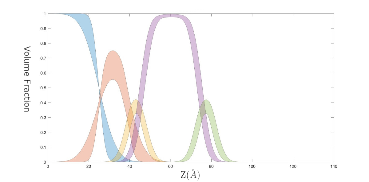
A Slightly Deeper Analysys - Plotting The Bayes Result as Volume Fractions

The model we're using here is built using Volume Fractions. It's convenient to be able to use these as outputs, so that the result of our Bayesian analysis in terms of the VF's of the various components can be visualised. To do this, we make our global output flag true....

outputVF = true;

Now we have an output for our VF's.

We want to see how these are distributed in our Bayesian analysis. All the information comes from our chain....

chain = results.chain;

Now, calculate the Volume Fractions for each sample of our Markov Chain, and store our VF outputs individual arrays....

% Find the size of the chain

nSamples = size(chain,1);

 

% We don't need to calculate all of it, just take a random 1000 points

% from the chain. Make a set of indicies...

samples = randsample(nSamples,1000);

Unrecognized function or variable 'randsample'.

 

% Make some empty arrays to store our data....

vfSi = []; vfOxide = []; vfHeadL = []; vfTails = []; vfHeadR = []; vfWat = [];

 

% Loop over all the samples...

for n = 1:length(samples)

% Take the n'th value from of set of indicies...

i = samples(n);

 

% Get these parameter values....

thisParams = chain(i,:);

 

% Run our model.....

[~,~,thisRes] = customXYDSPC(thisParams,2.07e-6,6.35e-6,1);

 

% Store them...

thisVfs = thisRes(:,2:end); % Column 1 is the z value...

 

% Add them to the arrays for storage...

vfSi = [vfSi ; thisVfs(:,1)']; % Note the transpose.....

vfOxide = [vfOxide ; thisVfs(:,2)'];

vfHeadL = [vfHeadL ; thisVfs(:,3)'];

vfTails = [vfTails ; thisVfs(:,4)'];

vfHeadR = [vfHeadR ; thisVfs(:,5)'];

vfWat = [vfWat ; thisVfs(:,6)'];

end

For each collection of volume fractions, we need the mean and the 65% Percentile.....

z = thisRes(:,1); nPoints = length(z);

 

% Make some empty arrays....

ciSi = []; ciOxide = []; ciHeadL = []; ciTails = []; ciHeadR = [];

avSi = []; avOxide = []; avHeadL = []; avTails = []; avHeadR = [];

 

% Make an inline function for calculating confidence intervals...

CIFn = @(x,p)prctile(x,abs([0,100]-(100-p)/2)); % Percentile function

 

% Work out average and confidence intervals...

avSi = mean(vfSi); ciSi = CIFn(vfSi,65);

avOxide = mean(vfOxide); ciOxide = CIFn(vfOxide,65);

avHeadL = mean(vfHeadL); ciHeadL = CIFn(vfHeadL,65);

avTails = mean(vfTails); ciTails = CIFn(vfTails,65);

avHeadR = mean(vfHeadR); ciHeadR = CIFn(vfHeadR,65);

 

% Make a plot.....

figure; hold on; box on

 

% In RAT, there is a useful function called 'shade' that we can use

% here.....

cols = get(gca,'ColorOrder');

shade(z,ciSi(1,:),z,ciSi(2,:),'FillColor',cols(1,:),'FillType',[1 2;2 1],'FillAlpha',0.3);

shade(z,ciOxide(1,:),z,ciOxide(2,:),'FillColor',cols(2,:),'FillType',[1 2;2 1],'FillAlpha',0.3);

shade(z,ciHeadL(1,:),z,ciHeadL(2,:),'FillColor',cols(3,:),'FillType',[1 2;2 1],'FillAlpha',0.3);

shade(z,ciTails(1,:),z,ciTails(2,:),'FillColor',cols(4,:),'FillType',[1 2;2 1],'FillAlpha',0.3);

shade(z,ciHeadR(1,:),z,ciHeadR(2,:),'FillColor',cols(5,:),'FillType',[1 2;2 1],'FillAlpha',0.3);

title('Volume Fractions');

.. and we are done.