Plotting Bayesian Analysis

A number of functions exist for plotting the results of Bayesian analysis. The problem and result used in this section were made using the DSPC Standard Layers example and a control object with the procedure set to DREAM.

MATLAB

% Run the DSPC standard layers example
controls = controlsClass();
controls.procedure = 'dream';
[problem, results] = RAT(problem, controls);

PYTHON

# Run the DSPC standard layer example
controls = RAT.Controls()
controls.procedure = 'dream'
problem, results = RAT.run(problem, controls)

Reflectivity and SLD

A simple reflectivity shaded plot can be displayed as follows:

MATLAB

bayesShadedPlot(problem, results)

PYTHON

RAT.plotting.plot_ref_sld(problem, results, bayes=65)

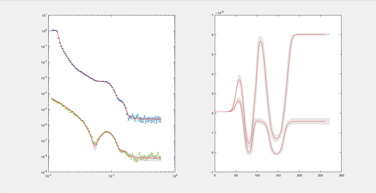
By default, this shows a standard reflectivity plot with a 65% shaded confidence interval.

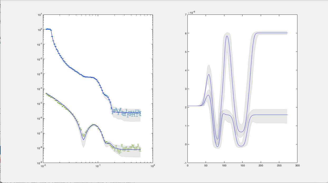
There are a number of options to customise the plot:

Interval - You can specify either the 65% or 95% confidence interval to display:

MATLAB

bayesShadedPlot(problem, results, 'interval', 95)

PYTHON

RAT.plotting.plot_ref_sld(problem, results, bayes=95)

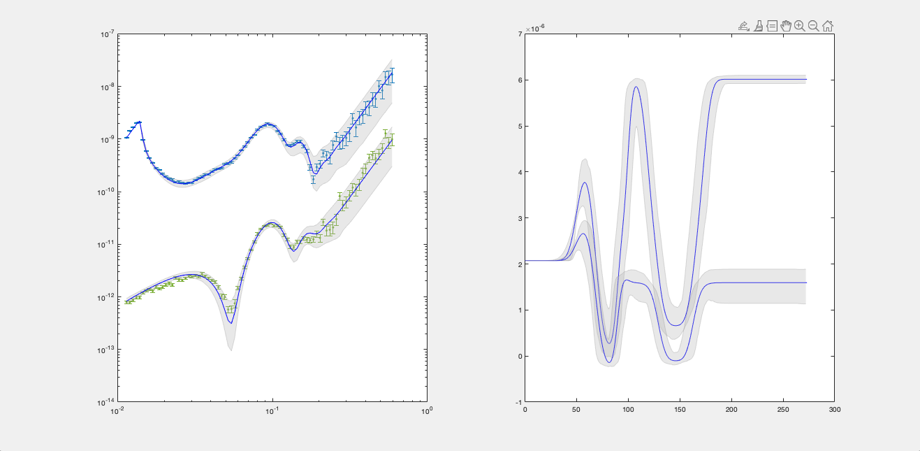
q4 - You can also specify a q4 plot for the reflectivity:

MATLAB

bayesShadedPlot(problem, results, 'q4', true)

PYTHON

RAT.plotting.plot_ref_sld(problem, results, bayes=65, q4=True)

Posterior Histograms

You can easily view the marginalised Bayesian posteriors from your analysis:

MATLAB

plotHists(results)

PYTHON

RAT.plotting.plot_hists(results)

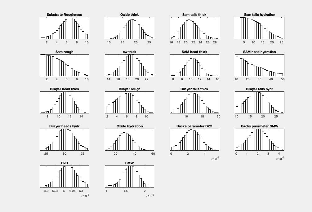
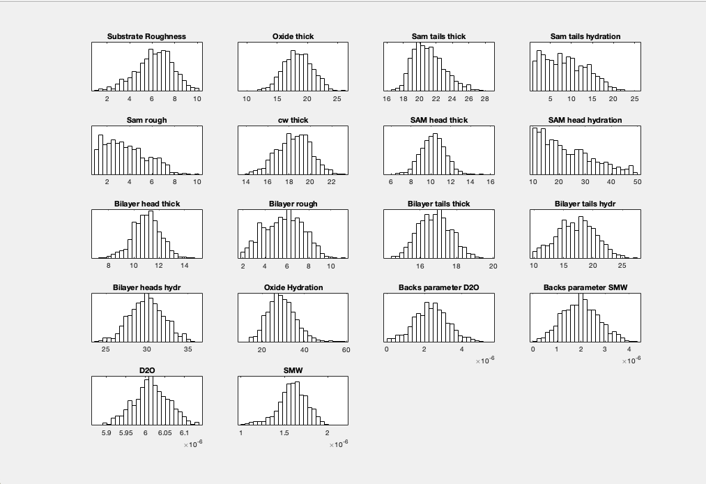
By default, the histogram plot function carries out a KDE smooth of the histograms. You can optionally choose no smoothing:

MATLAB

plotHists(results,'smooth',false)

PYTHON

RAT.plotting.plot_hists(results, smooth=False)

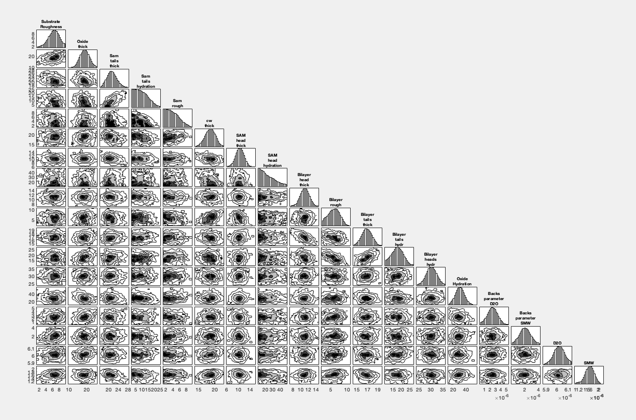
Corner Plots

To produce a corner plot, simply use the corner plot function:

MATLAB

cornerPlot(results)

PYTHON

RAT.plotting.plot_corner(results)

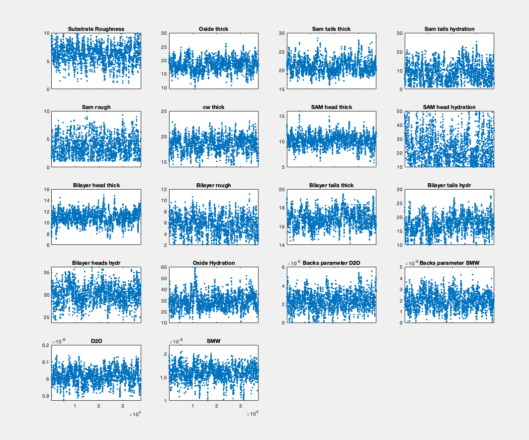
Chain View

Finally, you can check the integrity of your markov chain as follows:

MATLAB

plotChain(results);

PYTHON

RAT.plotting.plot_chain(results)