Bayesian Analysis#
RAT has two Bayesian algorithms available, Nested Sampling and DREAM.
These algorithms use statistical techniques to estimate the true value of fit parameters. The nested sampler also calculates Bayesian evidence, which may be used to compare hypotheses or models.
The central idea here is that the probability of a parameter \(X\)’s true value being \(x\) is related to its chi-squared fit: [1]
where \(I\) is the background information from the project. This means we can explore this probability (‘likelihood’) function to learn statistical information about the experiment and model.
Warning
This tutorial expects that you are familiar with setting up a project and controls; see the Introduction and project class tutorials.
Setting up a Bayesian analysis#
To set up the Bayesian algorithm itself, simply set the procedure in the Controls object
to either "ns" or "dream":
Each of these algorithms have their own controls settings, as all procedures do. See the Nested Sampling and DREAM pages for an outline of these.
This is sufficient to run the algorithm. However, you may also want to use information about your parameters in the optimisation. All parameters in the Project object (parameters, background & resolution parameters, scalefactors, bulk in/out, and domain ratios where applicable) can be given a prior which will be used in the algorithm. This prior represents our initial understanding of the parameter.
The options for the prior type are:
- "uniform": A uniformly distributed prior. Represents no initial knowledge about the true value of the parameter.
- "gaussian": A Gaussian (normal) distribution, with given mean and variance.
Represents that we have reason to believe the true value lies around some value \(\mu\) with variance \(\sigma^2\).
- "jeffreys": A Jeffreys’ prior, which represents no initial knowledge similarly to uniform, but is also invariant
to changes of scale.
For Gaussian priors, \(mu\) and \(sigma\) are given to represent the mean and standard deviation of the distribution.
You can give the prior (alongside \(mu\), and \(sigma\) if relevant) when you create the parameter:
% this Gaussian prior has a mean of 0 and standard deviation of 1
problem.addParameter('My new param', 1, 2, 3, true, "gaussian", 0, 1);
problem.addParameter('My scale param', 10, 20, 30, true, "jeffreys");
problem.parameters.append(name='My new param', min=1, value=2, max=3, fit=True, prior_type="gaussian", mu=0, sigma=1)
problem.parameters.append(name='My scale param', min=10, value=20, max=30, fit=True, prior_type="jeffreys")
You can also change these values in existing parameters, just as you would for the minimum, value, maximum, and fit.
Running and plotting a Bayesian analysis#
Running a Bayesian analysis is the same as running RAT normally. Here we’ll do a DREAM analysis on the project from the DSPC Standard Layers example:
[problem, results] = RAT(problem, controls);
disp(results)
problem, results = RAT.run(problem, controls);
print(results)
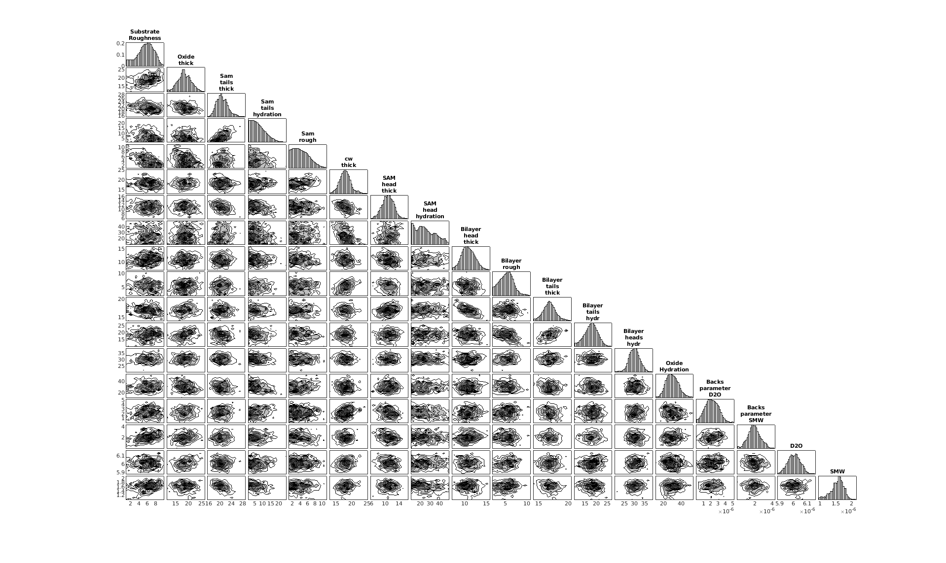
The results object contains additional results from the Bayesian analysis. The main thing you may want to do with this is create a corner plot of the posterior distributions:
cornerPlot(results);
RAT.plotting.plot_corner(results)
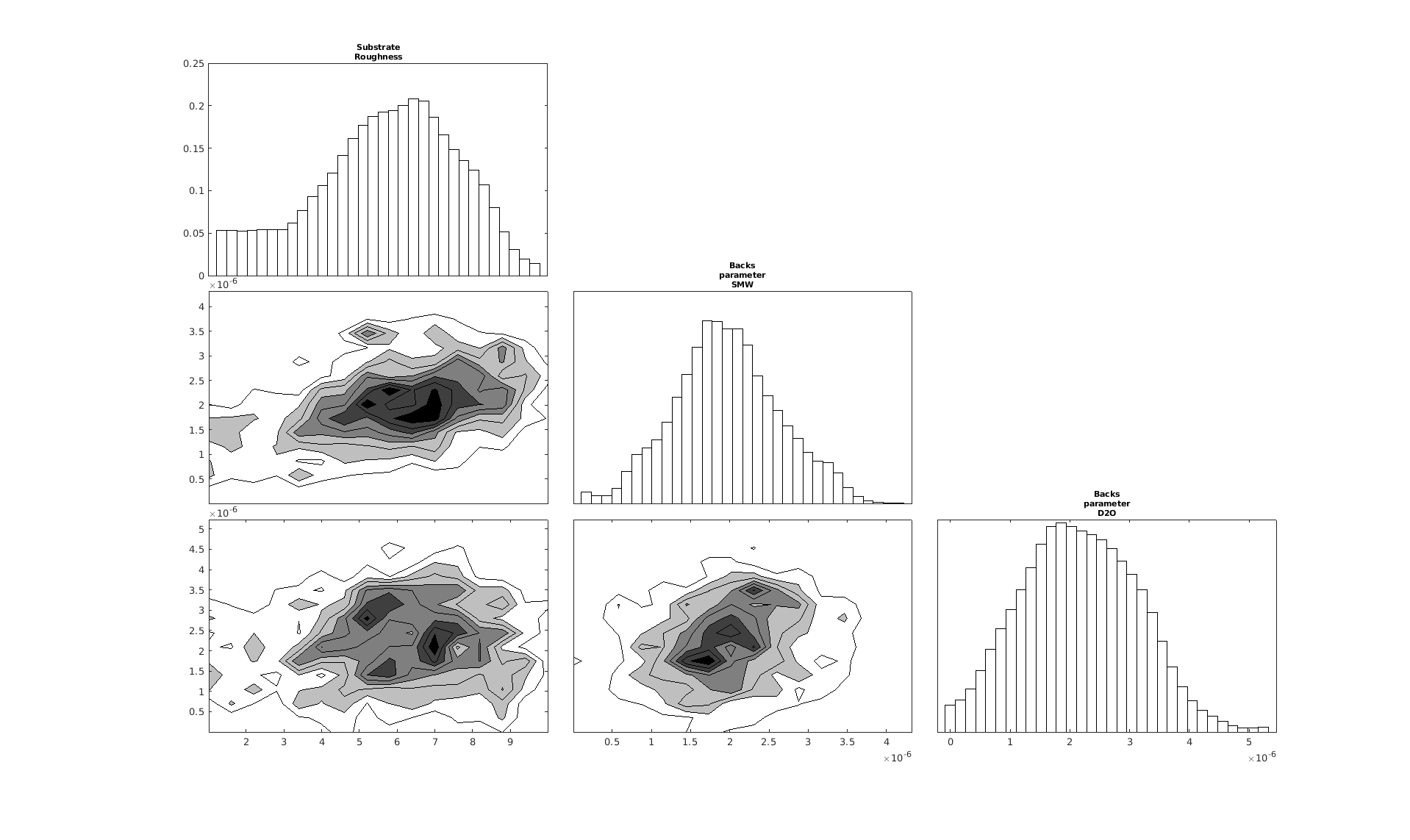
Note that you can specify some specific parameters to create a smaller, more focused corner plot:
cornerPlot(results, 'params', ["Substrate Roughness", "Backs parameter SMW", "Backs parameter D2O"]);
RAT.plotting.plot_corner(results, params=["Substrate Roughness", "Background parameter SMW", "Background parameter D2O"])
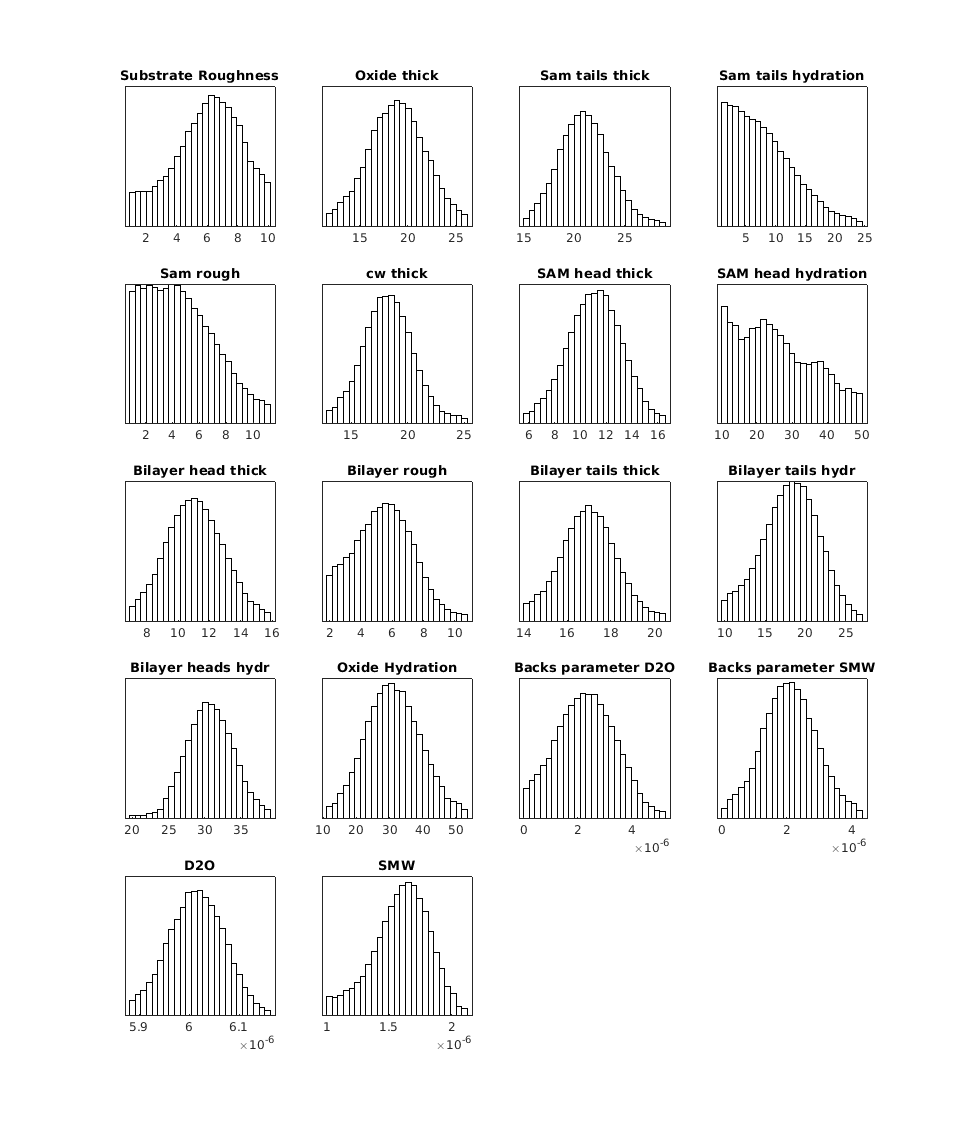
It is also possible to plot the histograms from the analysis as a grid:
plotHists(results);
RAT.plotting.plot_hists(results)
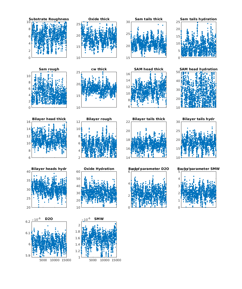
and also the Markov chains for each parameter:
plotChain(results);
RAT.plotting.plot_chain(results)